: added a paragraph about lowering the voxel update frequency for faster dynamic update. The
. They showed some nice results which attract me to implement the technique and my implementation runs at around 22~30fps (updated every frame) at 1024x768 screen resolution using a 256x256x256 voxel volume on my GTX460 graphic card. The demo program can be downloaded
which requires a DX11 GPU to run.
The step 1 and 2 can be done only once for static geometry while step 3 to 5 need to be done every frame. The following sections will briefly describe the above steps, you may want to take a look at the
first as some of the details will not be repeated in the following sections.
Voxelization pass
The first step is to voxelize the scene. I first output all the voxels from triangle meshes into a big voxel fragment queue buffer. Each voxel fragment use 16 bytes:
The first 4 bytes store the position of that voxel inside the voxel volume which is at most 512, so 4 bytes is enough to store the XYZ coordinates.
Voxel fragments are created using the conservative rasterization described in this
OpenGL Insights charter which requires only 1 geometry pass by enlarging the triangle a bit using the geometry shader. So I modify my
shader generator to generate the shaders for creating voxel fragments based on the material.
 |
| Scene before voxelize |
|
 |
| Scene after voxelize |
|
Octree building pass
I use a similar data structure that described in the
voxel cone tracing paper and
giga voxel paper with a large octree node buffer storing the octree/voxel node data (with 8 node grouped into 1 tile which described in the paper) and a 3D texture storing the reflected radiance and alpha from the direct lighting at that voxel (I assume all the surface reflect light diffusely so only 1 3D texture is used which is different from the paper storing incoming radiance).
Each octree node is 28 bytes with the first 4 bytes storing the child tile index with another 24 bytes storing the neighbor node byte offset from the start of the octree node buffer:
The child node tile index is also used to index the 3D texture brick(more details can be found in
voxel cone tracing paper about the texture brick) which store the reflected radiance of that octree node tile. And since I use 5 bits for store different bit flags for dynamic update, so my voxel volume can only be at most 512x512x512 large.
In the octree leaf node, it stores the voxel data directly which only use 16 bytes:
the first 4 bytes store the bit flag to indicate whether that voxel is created from static mesh so that it will not be overwrite by dynamic geometry. Also the 1 byte counter stored along with the voxel normal is used to perform averaging when different voxel fragments fall into the same voxel. The steps to perform atomic average can be found in the
OpenGL Insight Chapter.
So given the voxel fragment queue output from the previous steps, we can build the octree using the steps described in
OpenGL Insights Chapter and average the octree leaf node values when different voxels fall into the same node.
 |
| showing highest octree level |
|
 |
| showing the octree with the voxels |
|
Inject direct lighting pass
After building the voxelized scene, we need to add the lighting data into the data structure to calculate global illumination. First, we render the shadow map from the light's point of view. Then for each pixel of the shadow map, we can re-construct the world position of the shadow map texel and then traverse down the octree data structure to calculate the reflected radiance(assume reflected diffusely) and write it to the 3D texture bricks.

In my engine, I use cascade shadow map with 4 cascades, the last cascade is used to perform the light injection, with the slope scale depth bias disabled, otherwise, the re-constructed world position may not located exactly inside the voxel. Also, it is better to stablize the shadow map (in the demo, the position of the directional light is computed from view camera) in order to avoid flicking during cone tracing step when the camera moves. But after stablizing the shadow map, not all the voxels are filled with lighting data at 512x512x512 voxel resolution as the shadow map is not fully utilized...
This artifact will also occur when the shadow map resolution is low. Consider the the figure below, we have a directional light injecting lighting to the scene (which have a wall and floor).
As we launch one thread for each shadow map texel to determine which voxel get light injected, we can only inject light to 3 voxels(the white square in the figure) in the above case. While if the shadow map resolution is high enough, those 5 vertical voxels should all be injected with light.
Filtering pass
In order to perform cone tracing step, we need to filter the lighting data at the leaf node of the octree. The voxel lighting data is filtered anisotropically along the positive and negative XYZ directions. For example, in a 2D case(which is easier to explain and very similar to the 3D case), for each node tile, we will have 5x5 voxels which will be filtered to 3x3 voxels in the upper mip level like this:
To filter the center voxel(texel E in the figure) in the node tile in upper mip level along the +X direction, we need to consider the 9 texels (texel g, h, i, l, m, n, q, r, s in the figure) in the lower level, The texels are divided into 4 groups as the figure below:
in each group, we filter along the +X direction, for example in the upper left group, we first alpha blend the value in the +X direction and then average them to get the value for that group.
After calculate the values for all the 4 groups, we can compute the filtered center voxel value by repeating the above steps for the 4 group values.
But for the corner values(e.g. texel a, b, f, g) in a node tile we cannot access all the 9 texels to compute a filtered value as those values are in the neighbor node tile. So the group value are partially computed and store in the 3D texture first, then we rely on the transfer step described in the
cone tracing paper to complete the calculation. In other words, during the transfer steps, some of the filtered value is computed by first alpha blending the neighbor group values followed by averaging them, and other filtered value will be computed by averaging first followed by alpha blending. Although this calculation is not commutative, but this can reduce the number of dispatch passes to compute the filtered value with a similar result.
So we have 6 directional values for a filtered voxels. To get a sample from it for a particularly direction, we can sample it using the method like
ambient cube with 3 texture read (the following code is simplified):
float3 sampleAnisotropic(float3 direction)
{
float3 nSquared = direction * direction;
uint3 isNegative = ( direction < 0.0 );
float3 filteredColor=
nSquared.x * anisotropicFilteredBrickValue[isNegative.x] +
nSquared.y * anisotropicFilteredBrickValue[isNegative.y+2] +
nSquared.z * anisotropicFilteredBrickValue[isNegative.z+4];
return filteredColor;
}
Voxel Cone Tracing pass
After doing the above steps, we finally can compute our global illumination. We first consider the simple case for ambient occlusion, which need to compute the AO integral. We approximate it by partitioning the integral with several cones:
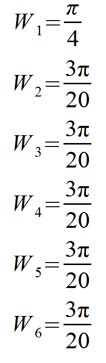
Where each partition need to multiply with a weight W. In my implementation, 6 cones are traced with 60 degree over the hemi-sphere in the following direction (Y-axis as the up vector):
each with a weight W:
Then to calculate the visibility inside one cone, we take multiple samples from the filtered 3D texture bricks along the cone direction:
But, the remaining problem is to determine the sampling position. Since we manually filter the 3D texture bricks, the hardware quadrilinear interpolation will not work. So to avoid performing the quadrilinear interpolation manually, It is better to make sampling position located at each mip level, having voxel size equals to the cone width at that position. This position is calculated by assuming the shape of voxel is sphere rather than cube(which is easier to calculate) as follows:
Then the sampling location can be calculated given the cone origin, cone angle, trace direction and voxel radius with some simple geometry. And here is the voxel AO result:
 |
| AO result using 512x512x512 voxel volume |
Next, for diffuse indirect illumination, the calculation is very similar to AO:
The indirect diffuse calculation is done using the same cones as the AO so that both the indirect diffuse and AO can be calculated at the same time:
Finally, we calculate the indirect specular, where cone is traced in the reflected view direction along the surface normal. The cone angle is depends on the glossiness,
g, of the material, currently I use the following equation to calculate the angle:
The glossiness is limited to a range so that the cone angle will not be too narrow to avoid stepping through thin walls. Here is the result of indirect specular:
In my engine, I use a light pre-pass renderer, so for the opaque objects, I calculate the indirect lighting by rendering a full screen quad after the lighting pass which is then blend on top of the direct lighting buffer using the following blend state:
With the value of AO store in alpha channel. this can apply AO to both the direct and indirect lighting. Sometimes different AO intensity is need for the direct and indirect light, this blend state can be used instead:
which apply the alpha blending to only the direct lighting and the indirect AO is applied inside the shader.
When filtering mip map directionally from the leaf node, normal direction is not taken into account, which results in more light leaking for thin objects as below. And this artifact can be hidded slightly with the AO value calculated in cone tracing:
 |
| light leak through thin geometry |
|
 |
| apply the AO can only hide the leaking a bit |
|
Dynamic update
To make the indirect illumination calculation faster, 5 ways are used to speed up the calculation a bit.
First, when the scene is initialized, the first 4 steps that described in the overview section are performed for all the static geometry. Then in every frame, we re-calculate all the 5 steps for voxels that affected by dynamic objects. So, only dynamic objects will be voxelized every frame (while static voxels are already stored in the octree and we don't overwrite those data which can be identified by bit flag stored in the node). Those dynamic voxel fragments are appended to the end of the octree node buffer which can be cleared easily. Also, we need to reset the static octree node neighbor offset which points to dynamic nodes, and those static nodes that affected by dynamic voxels in previous and current frame need to re-filter again. Those nodes are found by dispatching threads for all the nodes and queue those node index into another buffer. So only those with changed value will be re-calculated.
Second, for voxelizing the dynamic geometry, the InterlockedMax() function is used to compute both the diffuse and normal for the octree voxel which is faster than performing an atomic average. Note that using InterlockedMax() function for the normal will decrease the lighting quality if the voxel volume is
at a small size(e.g. 256x256x256). You can see the artifact in the below figure:
 |
| Reflect light using an average voxel normal |
|
 |
| Reflect light using InterlockedMax() voxel normal. |
|
So I only use InterlockedMax() function for normal in the dynamic geometry and keeping the static geometry computing an average normal. That is why you can see the octree voxel data structure(in octree building pass section) store a 1 byte counter along with the normal but not other attributes.
Third, I perform a view-frustum culling when injecting the direct lighting into the octree because there is no point to filter the light that is far from the camera where we never sample it from the current point of view. An extended frustum is calculated from the current camera (refer to the figure below) for culling.
This frustum is simply moving the camera backward a bit with increased far plane using the same field of view. The extended distance is calculated by the maximum cone tracing distance (I limited the cone tracing distance in the demo, which lost the ability to sample from far objects like the sky) and the filtered voxel size.
Fourthly, I perform the cone tracing pass at half resolution of the screen resolution. However, this result in visible artifact when up-scaling to full resolution especially at the edge of the geometry (the strength of the indirect lighting in the following screen shots are increased to show the artifact more clearly).
 |
| up-sample with only bilinear filtering |
So, I first decided to just fix those pixels by finding them with an edge detection filter using depth buffer.
 |
| perform an edge detection pas |
And then perform cone tracing at those pixel again at full resolution:
 |
perform the cone-tracing again in
the edge pixel at full resolution |
Some of the artifacts are gone, but the frame rate drops a lot again...
So, my second attempt is to just simply blur those pixels (averaging with the neighbor pixel). The quality of blurring is not as good as re-compute the cone tracing, but it is much faster.
 |
| up sample with blurring at edge |
|
 |
| cone tracing at full resolution for reference |
|
Lastly, The voxel world can be updated at a different frequency than the render frame rate. By assuming the light source/dynamic models are not moving very fast, we can take advantage of the temporary coherency and perform the voxelization at a lower frequency, say update at every 5 frames. We can trade the accuracy of the voxels for update speed, but this may result in the artifact shown below:
 |
The voxel model is lag behind the triangle
mesh due to the lower update frequency |
Conclusion
The advantage of voxel cone tracing is to compute the GI in real-time with both the dynamic lighting and geometry. Also the specular indirect lighting gives a very nice glossy effect. However, it uses lots of the processing power/memory and quality of lighting is not as good as the baked solution. In my implementation, I can only use 1 directional light to compute single bounce indirect lighting. And there are still room to improve in my implementation as fewer cones can be used for tracing, using the depth buffer for view frustum culling, better up-sampling when performing cone tracing and divide the voxels into several regions to handle a larger scene like Unreal Engine does. But there is never enough time to implement all that stuff... So I decided to release the
demo at this stage first. In the demo, I have added some simple interface (for changing stuffs like the light direction, indirect lighting strength) for you to play around with. Hope you all enjoy the
demo.
Finally, I would like to thanks Kevin Gadd and Luke Hutchinson for reviewing this article.
References